Laplacian Surface Editing (LSE)

In this post, I'll be discussing surface deformation, differential geometry, least squares, and sparse linear linear systems.

In Laplacian surface editing (LSE), the goal is to deform a mesh surface while minimizing changes to its differential geometry. Differential geometry is really neat: position data is defined based on the weighted average differences between a given point and its neighbors. For a vertex $v_i$, we define its differential coordinate:

$$
\begin{equation}
\delta_i = v_i - \frac{1}{d_i}\sum_{j \in N_i} v_j,
\end{equation}
\label{eq:deltai}
$$

where $N_i$ is the one-ring neighborhood of $v_i$ and $d_i$ is the number of elements in $N_i$. For updated mesh data that may differ from the initial state, I'll use the prime symbol: $v_i'$. I'll refer to $\delta_i'$, which is computed the same way, only with $v_i'$ and $v_j'$ substituted in Equation$~\ref{eq:deltai}$ appropriately.

We could certainly compute $\delta_i$ for all $i$ in our mesh directly, but the linear algebra way is prettier. A 3D mesh $M$ with $n$ vertices has vertex matrix $V_{n \times 3}$, adjacency matrix $A_{n \times n}$ ($A(i,j) = 1$ if vertices $i$ and $j$ share an edge, $0$ otherwise), and diagonal matrix $D_{n \times n}=$diag$(d_1,...,d_n)$. Then using $L= I - D^{-1}A$, we can find $\Delta = \lbrace \delta_i \rbrace = LV$. $L$ is called the Laplacian operator of $M$ with adjacency $A$. Computing $LV$ fills $\Delta$'s rows with the same thing as Equation$~\ref{eq:deltai}$. An importing thing to note is $L$ has rank $n - 1$, which means we can recover $V$ from $\Delta$ as long as we fix at least one vertex position ($v_i' = u_i, i \in \lbrace m,...,n \rbrace, m < n$) and solve a linear system. A least squares approach has been observed to be preferable to exact solvers, so we end up with an error functional:

$$
\begin{equation}
E(V') = \sum_{i=1}^{n}||\delta_i - \delta_{i}'||^2 + \sum_{i=m}^{n} ||v_i' - u_i||^2
\end{equation}
\label{eq:lseerror}
$$

Differential coordinates are sensitive to linear transformations, so in order to get an agreeable deformation across $V'$ having only manually fixed a small set of vertex positions, the LSE authors seek to find transformations for each vertex $T_i$ that minimize Equation$~\ref{eq:lseerror}$ based on $V'$. That is, $T_i$ is a function of $V'$, and the error functional becomes:

$$
\begin{equation}
E(V') = \sum_{i=1}^{n}||T_i(V')\delta_i - \delta_{i}'||^2 + \sum_{i=m}^{n} ||v_i' - u_i||^2
\end{equation}
\label{eq:lseerror2}
$$

The next insight is that the coefficients of $T_i$ are a linear function in $V'$, and solving for $V'$ implies finding $T_i$ because $E(V')$ is a quadratic function in $V'$. Are we having fun yet?!!

We're all about differentials here, so it makes sense to try and find $T_i$ based on $v_i$'s neighbors:

$$
\begin{equation}
\min_{T_i} \Big( ||T_i v_i - v_i'||^2 + \sum_{j \in N_i} ||T_i v_j - v_j'||^2 \Big)
\end{equation}
\label{eq:lsetimin}
$$

We need to constrain $T_i$ in order to avoid finding a membrane solution for $E(V')$. Anisotropic scaling is out because it can remove the normal component from the differential coordinates. Translation in $T_i$ is permitted by using homogeneous coordinates ($v_i = (x_i, y_i, z_i, 1.0)$), and the linear portion should only use isotropic scaling and rotations. Matrices with only isotropic scaling and rotation can be expressed as $T=s\exp{H}$, where $H$ is a skew-symmetric matrix (these emulate cross products with a vector: $Hx = h \times x$). They use some other fancy properties of $3 \times 3$ skew matrices and come up with:

$$
\begin{equation}
s\exp{H} = s(\alpha I + \beta H + \gamma h^T h)
\end{equation}
\label{eq:tderive}
$$

They observe that only $s, I$, and $H$ are linear in the unknowns of $s$ and $h$, while $h^Th$ is quadratic. A linear approximation of the class of constrained transformations gives them:

$$
\begin{equation}
T_i =
\begin{pmatrix}
s & -h_3 & h_2 & t_x \
h_3 & s & -h_1 & t_y \
-h_2 & h_1 & s & t_z \
0 & 0 & 0 & 1
\end{pmatrix}
\end{equation}
\label{eq:tapprox}
$$

The vector of unknowns in $T_i$ is $(s_i, h_i, t_i)^T$, and the goal is to minimize:

$$
\begin{equation}
||A_i (s_i, h_i, t_i)^T - b_i ||^2
\end{equation}
\label{eq:shtmin}
$$

The linear least-squares problem is solved by:

$$
\begin{equation}
(s_i, h_i, t_i)^T = (A_i^T A_i)^{-1} A_i^T b_i ,
\end{equation}
$$

where $A_i$ contains the positions of $v_i$ and its neighbors and $b_i$ contains the positions of $v_i'$ and its neighbors. And that's that!

But not really. $T_i$ is only an approximation of isotropic scale + rotation transformations, and it falls apart with large angle rotations. Plus, anisotropic scales are cool! What's wrong with that? The solution is to compute $T_i$ with $V, V'$, then update $\delta_i$ depending on what's desired in the surface edit, then solve the system again. For very large angles of rotation, there's an approximate reconstruction method that can be used first, then refined with the LSE technique.

If you couldn't tell, there's a good amount of work required in order to get to a point where you can finally solve a system $Ax=b$ and get the results you need. The explanation I've given here wavers towards the end, so I urge you to dive into the paper and see it done properly. My main goal here is to introduce the technique and demonstrate what goes into executing it. In order to use LSE on your mesh, you'll need a way to specify regions of interest (ROI) on which LSE operates. A region of interest contains:

• a set of static anchor vertices remain fixed in position,
• a set of handle anchor vertices are transformed into desired positions,
• a set of in-between vertices that are fully bounded by static anchors.

With that out of the way, let's see how this looks:

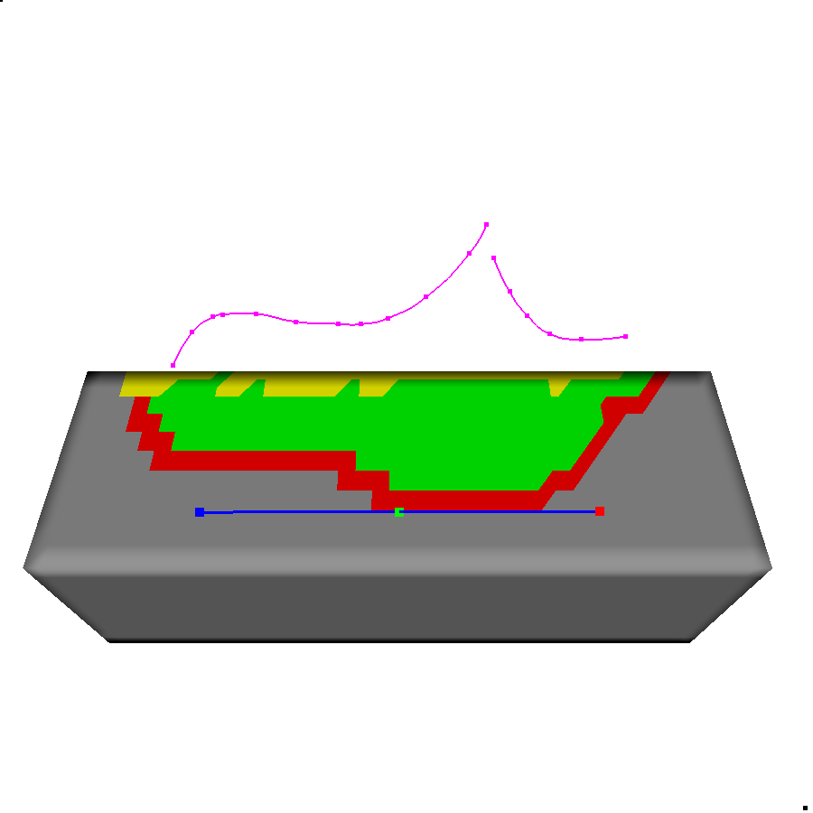
This is from a much older version of my implementation, but it's a nice demo. The faces in red represent static anchors, which wrap around the other side of the mesh to form a complete boundary. The faces in green represent vertices contained within the static anchors, and the vertices in yellow represent the handle anchors to be transformed. This implementation follows the style of SilSketch, which automates ROI creation and handle deformation for LSE based on a mesh's silhouette and the size of input strokes.

The output of the ROI and strokes above give us:

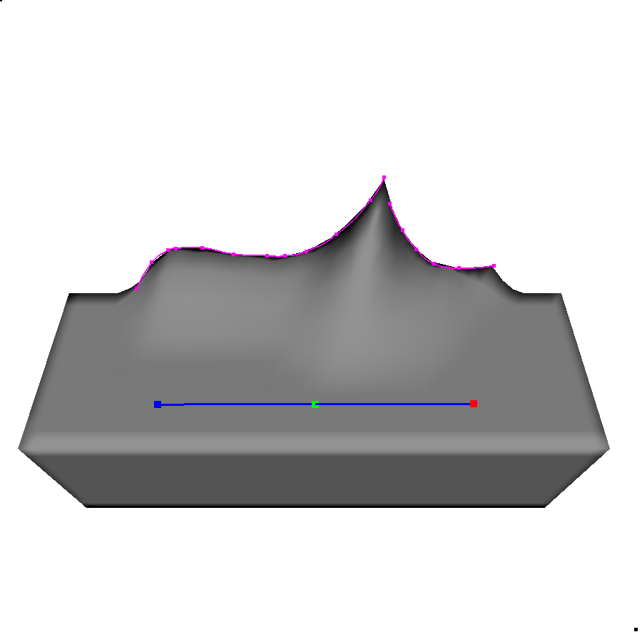
Now combining surface deformations with skeletal deformations (skinning) gets tricky, but that's another post :)