Implicit Skinning, Part 1

This is going to cover the paper, ""Implicit Skinning: Real-Time Skin Deformation with Contact Modeling,"" from Rodolphe Vaillant et al., and the work on which it builds (implicit surfaces, HRBFs). The prerequisite list is long, but here's a start:
- functional analysis
- radial basis functions
- Hermite and Banach spaces
- Hermite data (for our use: positions and normals)
- space operators - composition of several HRBFs into one
Overview
One of the better overview figures I've seen:
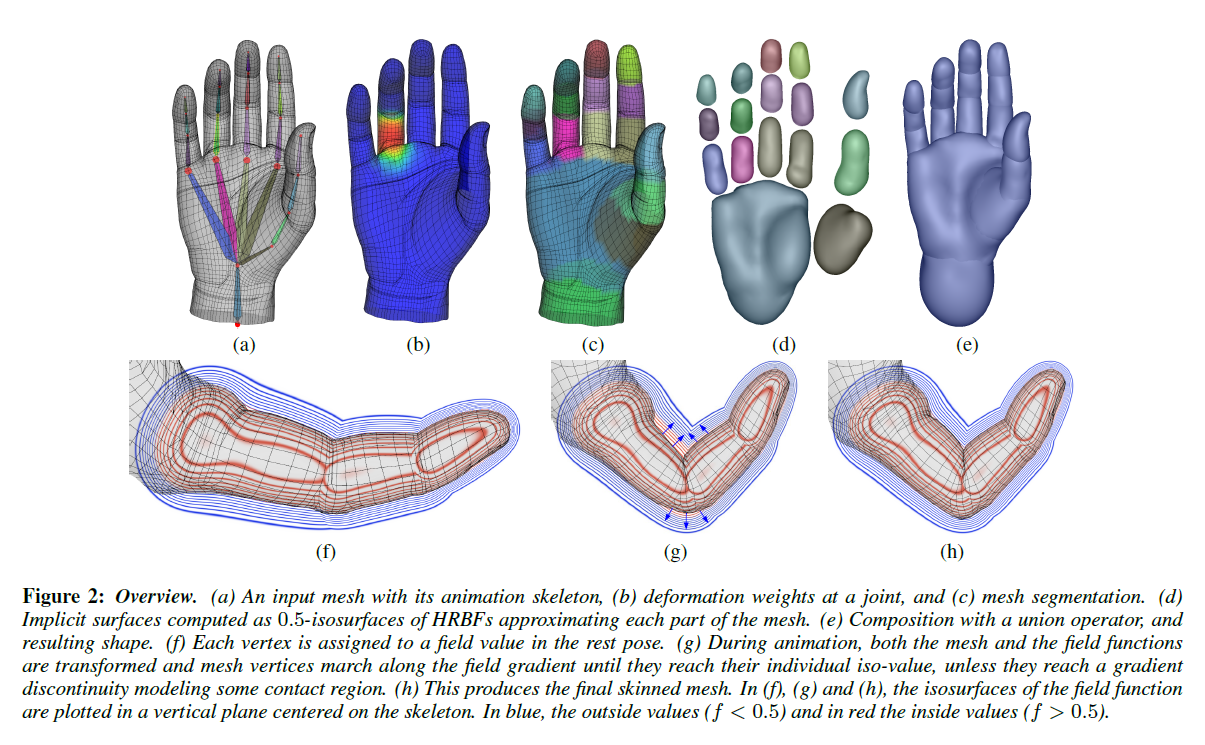
Given a prepared mesh (surface, skeleton, skin weights), they:
- Segment the mesh using the skin weights
- Create implicit surfaces out of each segmented mesh region
- Union the surfaces back together and normalize the function
- Save each vertex's offset in the field (a value of 0.5 in the field is the implicit surface, so vertices will have very tiny offsets from that. Why? The point sampling method used produces implicit surfaces (HRBFs) that very much resemble the mesh segment, making the distances between the original vertices and the implicit surface very small).
Then for animation, they:
- Skin the mesh using plain old LBS (or DQS)
- Transform the implicit surfaces using the bone transforms. Scalable or curved bones aren't supported by default
- Union them together and sample it into a 3D texture
- Project the post-skinned vertices until they reach their stored offset or they reach a discontinuity in the field. The discontinuity represents a contact surface with another part of the mesh.
- Perform some relaxation and smoothing steps along with the vertex projection to produce various kinds of contact surfaces (bulge, fold, etc.)
Pretty cool, right? The method allows the mesh to detect self-intersections and compensate for them with real-time adjustments.
Field construction
From the paper:
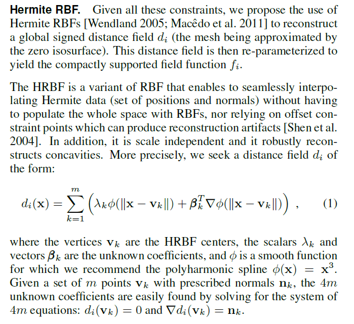
To find the HRBF centers, they use Poisson disk sampling[1] with a target of 50 samples per sub-mesh. They also include two additional HRBF centers. These lie on the bone axis, one on each side. Each center is the same distance past the bone's endpoint as the closest vertex to the joint. The normal is pointed outward, away from the bone and mesh.
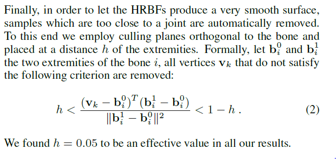
Having centers that are too close to the bone will cause problems, so they filter that out too:
Re-parameterization
Here, they transform the distance function $d_i$ (for each bone $i$ and its corresponding sub-mesh) and turns it into a compactly supported function $f_i$:
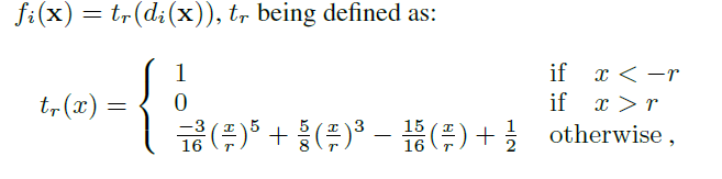
where $r$ is the max distance between the HRBF centers and the bone. The result is $f_i(0.5)$ corresponds to the surface, and each vertex can track its own offset to be used for skinning.
Why is compact support so important for $f_i$? Well, it lets them be sampled neatly into finite 3D textures for our exploitation enjoyment!
Composition of $f_i$ into $f$
They find a new field function $f_k$ = $g_k$ ($f_i$, $f_j$) for each neighboring pair of bones $i,j$ using a binary composition operator. $g_k$ can vary, but for an example they use:
$$
\begin{equation}
g_k = \max(f_i, f_j)
\end{equation}
\label{eq:binaryoperator}
$$
Changing the operators $g_k$ will produce different behavior around joints -- use of Equation $\eqref{eq:binaryoperator}$ will cause the skin to both fold and avoid elbow collapse. The variance here allows for a specialized approach for each joint type. Elbows might be treated differently than necks or shoulders.
The final field $f$, which is the implicit surface version of the input mesh, is the union of all $f_k$. Choice of composition can vary here, but for demonstration, they choose Ricci's max operator:
$$
\begin{equation}
f = \max_{k} f_k
\label{eq:riccimax}
\end{equation}
$$
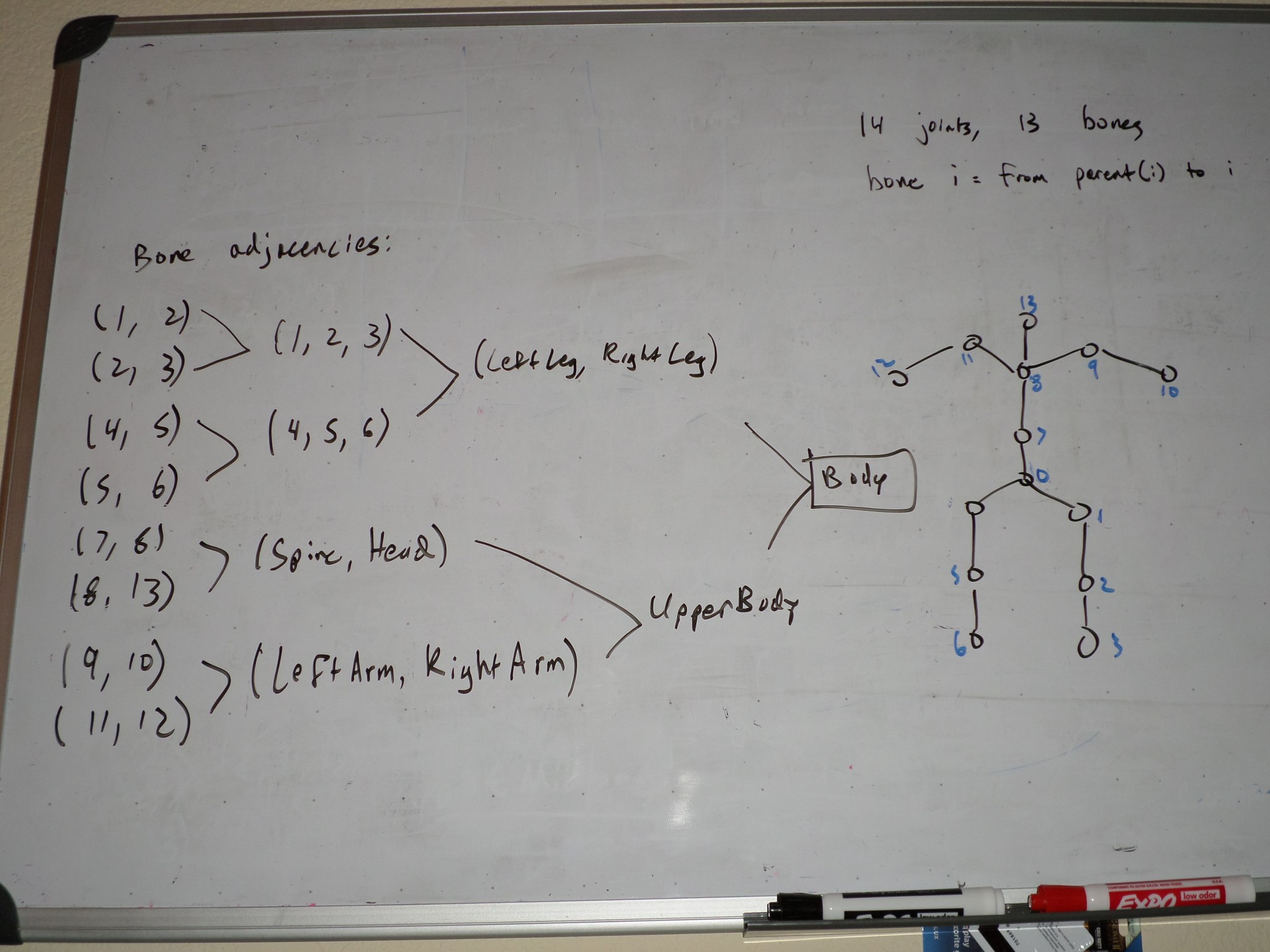
Consider the composition of these implicit surfaces into a more complex surface. Equation $\eqref{eq:riccimax}$ combines the set of $f_k$, which are operators that combine implicit surfaces adjacent according to the skeleton structure. The result is a fully realized, compactly supported implicit surface over the entire mesh. In the next paper, $f$ is composed using a tree structure. Not exactly like this, but something to the effect:
Blending operators
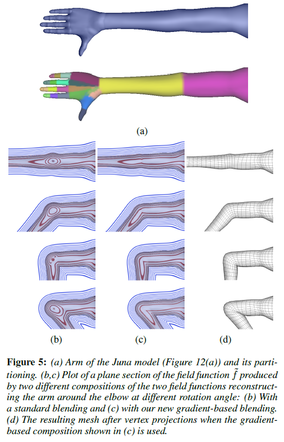
Implicit modeling and rendering uses smooth blending operators to control the behavior of adjacent implicit surfaces. In a sense, they control the smooth skinning of implicit surfaces much like the weights and blending method control the smooth skinning of polygon meshes. By default, traditional smooth blending operators may not produce desirable results for the implicit skinning method. Instead, the use of a gradient-based composition operator will react to a function of the angle $\alpha$ between the gradient computed at point $p$ in $f_i$ and $f_j$. This approach interpolates between a union operator and a blending operator based on $\theta(\alpha)$. If $\alpha=\theta_u$, a union is used. If $\alpha=\theta_b$, a blend is used. Otherwise, an intermediate local blend is used. See below for a comparison between the smooth blending operators and gradient-based composition operators:
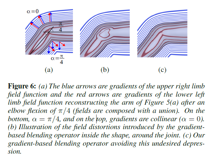
There's a bit of small-angle approximation going on: by observing that $\alpha$ is close to the rotation angle between the bones $i,j$ in the folding region of the mesh, and that $\alpha$ is close to $0$ for the outer mesh region, the authors can define $\theta(\alpha)$ (really, they're defining $\theta_u$ and $\theta_b$) in a particular manner to produce desired skinning results for different joints and regions. However, the existing gradient-based composition operator is unsatisfactory because it creates a depression around the joints. Because the gradient vectors are so critical for vertex projection, they make adjustments to the composition to make it suitable for implicit skinning. The figure below contains a visual comparison of $\alpha$ on the inner and outer fold of a surface, as well as the difference between the default and modified gradient-based operators.
And here is how the gradient-based operator is defined:
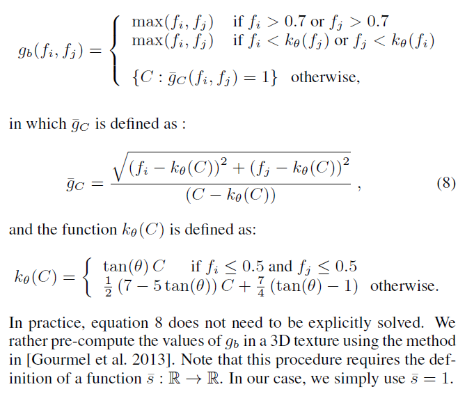
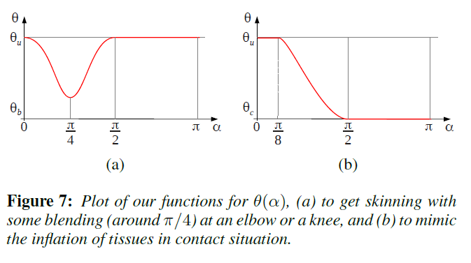
For finger joints and other situations where implicit surfaces readily make contact, a gradient-based bulge-in-contact operator is used, which interpolates between a union and contact surface surrounded by bulge. In addition to operator, choice of $\theta(\alpha)$ drastically impacts the skinning simulation:
Skinning
Vertex projection
The first part is easy: skin the mesh vertices using LBS or DQS. The implicit surfaces $f_i$ will also need to be transformed to match their bones and re-composed into $f$. Side-note: can this be done without resampling into the textures? After the vertices have been transformed, they need to be adjusted such that their skinned iso-value with respect to $f$ is the same as their bind iso-value. They use Newton iteration to do this:
$$
\begin{equation}
v_i \Leftarrow v_i + \sigma (f(v_i) - iso_i) \frac{\nabla f(v_i)}{|| \nabla f(v_i) ||^2}
\label{eq:vertexprojection}
\end{equation}
$$
They note $\sigma=0.35$ as a compromise between convergence and accuracy.
To prevent self-intersections, the iterations halt when it detects a gradient discontinuity in the scalar field. The precise check used is angle$(\nabla f (v_i^{current}),\nabla f (v_i^{last})) > 55^{\circ}$.
Tangential relaxation
Projection iterations are interleaved with a tangential relaxation step, moving each vertex towards the weighted centroid of its neighbors. Given $v_i$, let $q_{i,j}$ be its one-ring neighbors projected onto the tangent plane. We compute $\Phi_{i,j}$, the barycentric coordinates of $v_i$ such that $v_i = \sum_{j}{\Phi_{i,j} $q_{i,j}}$ using the mean value coordinate technique. The relaxation step moves a vertex tangentially to the local surface:
$$
\begin{equation}
v_i \Leftarrow (1 - \mu) v_i + \mu \sum_{j}{\Phi_{i,j} $q_{i,j}}
\label{eq:tangentrelax}
\end{equation}
$$
$\mu \in [0, 1]$ controls the relaxation amount and improves the vertex distribution. They control $\mu$ so that vertex displacement decreases with the distance to the iso-surface:
$$
\begin{equation}
\mu = \max(0, 1 - (|f(v_i) - iso_i | - 1)^4)
\label{eq:mu}
\end{equation}
$$
Laplacian smoothing
Finally, Laplacian smoothing is applied only to vertices in contact regions to smooth deformations from the union operator, which can introduce sharp features:
$$
\begin{equation}
v_i \Leftarrow (1 - \beta_i) v_i + \beta_i \widetilde{v_i}
\label{eq:laplaciansmooth}
\end{equation}
$$
where $\widetilde{v_i}$ is $v_i$'s one-ring neighborhood centroid, and $\beta_i$ controls the smoothing amount. Vertices stopped at gradient discontinuities are given $\beta_i=1$, all others are given $\beta_i=0$. Diffusion is used to smooth $\beta_i$ over the mesh, then Equation $\eqref{eq:laplaciansmooth}$ is applied. Since this step requires knowing whether the vertices were stopped, it must occur after the interleaved vertex projection/tangential relaxation steps.
Implementation
CUDA is used to parallelize all of the skinning steps:
- dual quaternion skinning
- vertex projection
- tangential relaxation
- localized Laplacian smoothing
From what I can see in their source code, all of these steps are done with CUDA kernels and routines as opposed to OpenGL shaders. Of course the geometric skinning step could be done with vertex shaders, but I'm not so sure about the vertex projection or tangential relaxation. And since the implicit stages require CUDA, it makes sense to do skinning in CUDA as well for streamlined data access. In an OpenGL shader, you would have to do the typical shader setup:
- Create VBOs for the mesh data. Struct of arrays or array of structs.
- Create a VAO to preserve the vertex attribute bindings.
- Set up a transform feedback (XF) buffer to catch the output of vertex processing (skinning shader)
- Provide a vertex shader that corresponds to the VAO/VBO/XFB
- Render the mesh. For performance, disable the rasterizer and use GL_POINTS so the XFB indices are consistent with the mesh input.
- Use the XFB's contents as input for the next two steps.
Mixing CUDA and OpenGL made me a little nervous at first, but there's plenty of info out there on how to do it. Two of my favorite finds so far are:
- What Every CUDA Programmer Should Know About OpenGL - a series of slides from GTC 2009. It includes examples on how to bind buffers to CUDA handles for both textures and VBOs.
- The NVIDIA DesignWorks samples includes an example of CUDA/OpenGL interop.
With these resources, it's not too far-fetched to attach CUDA stages to the existing OpenGL-based pipeline. I already perform steps 1 through 5 in the list above. Step 6 would involve registering the transform feedback buffers with CUDA and set up similar routines for the implicit skinning steps.
To perform the fancy parts of implicit skinning, we depend on each bone's implicit surface being compactly supported and accessible (we don't want to evaluate complex HRBFs directly in the vertex shader!). We require the same for the 3-dimensional composition operators that determine what value to return for two field function values and the angle between the gradient at each field's point. The field functions and composition operators are sampled into $32^3$ and $128^3$ 3D textures, respectively, using trilinear interpolation. Composition operator texture dimensions are provided by $(f_1, f_2, \tan(\theta))$, $f_1$ and $f_2$ being the scalar field values $\in [0, 1]$ and $\tan(\theta)$ being the angle between the gradients at those values.
Results
Implicit skinning is a very neat technique. The core idea offers a robust method for detecting and controlling self-intersecting mesh regions that can occur during animation. However, it has drawbacks:
- The method depends on the quality of the provided skin weights.
- Large angle bends are considered harmful - vertex will translate so far past their normal range that the gradient discontinuity detected will cause it to push through to the other side.
- Vertices are subject to flickering while the mesh is in motion. It's possible for the vertex to, at times, to end up on alternate sides of a gradient discontinuity during animation, causing the flicker
- Can lead to overstretching on the outside of joint bends
There's a lot that the authors do to fix these issues, which will be covered in more depth in part 2!
from ""Poisson Disk Point Sets by Hierarchical Dart Throwing (White, Cline, and Egbert): A Poisson-disk point set is defined as a set of points taken from a uniform distribution in which no two points are closer to each other than some minimum distance, r. The point set is said to be maximal if there is no empty space left in the sampling domain where new points can be placed without violating the minimum distance property. Poisson-disk point sets are useful in a number of applications, including Monte Carlo sample generation, the placement of plants and other objects in terrain modeling, and image halftoning. ↩︎